---
title: "Nearest-Neighbor Gaussian Process (NNGP): Joint Density, Sampling, and Prediction"
author: Fabian R. Ketwaroo
date: last-modified
format:
html:
toc: true
toc-depth: 3
theme: cosmo
code-fold: show
code-tools: true
bibliography: sIPMrefs1.bib
---
```{=html}
<!---
danielturek.github.io/nngp/nngp_RW_sampler/demo.html
-->
```
Back to [Index](https://danielturek.github.io/nngp/analysis/index.html)
In this vignette, we provide a practical, end-to-end guide to implementing **Nearest-Neighbor Gaussian Process (NNGP)** models within a Bayesian hierarchical framework in `NIMBLE` [@de2017programming] and our package `BayesNSGP`. We begin with a brief conceptual overview of standard Gaussian Processes (GPs) and detail how the NNGP approximation circumvents the traditional computational bottlenecks of large-scale spatial modeling.
Using `NIMBLE` together with `BayesNSGP` custom backend extensions, we walk through the complete workflow of a spatial analysis:
1\. **Data Generation**: Simulating a spatially autocorrelated surface and generating observed Poisson counts.
2\. **Model Specification**: Constructing the neighborhood topology and embedding NNGP joint densities directly into BUGS code.
3\. **MCMC Optimization**: Configuring and comparing three distinct sampling strategies—the default joint block sampler (`RW_block`), independent single-node random walks (`RW`), and `BayesNSGP` custom local neighborhood sampler (`RW_NN_GP`).
4\. **Out-of-Sample Prediction**: Executing fast, posterior predictive interpolation at unobserved locations using the sequential conditional structure of the NNGP.
By the end of this vignette, readers will understand how to use `BayesNSGP` to construct, fit, and predict from NNGP-based spatial models in `NIMBLE`, and how these tools can be integrated into a broad range of hierarchical ecological models.
# 1. Introduction
## 1.1 Gaussian Process (GP)
A Gaussian process (GP) [@williams2006gaussian] is a non-parametric probabilistic modeling framework that defines a probability distribution over possible functions. Formally, for location $s$,
$$ \omega(s) \sim \text{GP}(m(s), K(s,s^{\prime}))$$
where $m(s)$ is the mean function and $K(s,s')$ is the covariance function between any two locations ($s$ and $s^{\prime})$. The mean function gives the expected value of the process at location $s$, while the covariance function specifies the dependence between locations and controls the smoothness and variability of functions drawn from the GP. Critically, for any finite set of spatial locations $H= \{s_1,\ldots,s_M\}, \boldsymbol{\omega} = (\omega(s_1), \ldots ,\omega(s_M))^\top$ follows a multivariate normal (MVN) distribution
$$\boldsymbol{\omega} \sim \text{MVN}(\boldsymbol{m}, \boldsymbol{K})$$
with a mean vector $\boldsymbol{m} = [ m(s_1), \ldots, m(s_M)]^\top$ and covariance matrix $\boldsymbol{K}$ with entries $K(s_i, s_j)$. This finite representation enables practical computation of GP, as the MVN distribution is well understood mathematically and computationally tractable. Consequently, GPs provide a powerful framework for modeling residual spatial autocorrelation, naturally capturing complex, nonlinear dependence structures in space and yielding reliable parameter estimates with associated uncertainty.
Here, we assume $m(s) =0$ and employ an exponential covariance function:
$$ K(s_i,s_j) = \sigma^2 \exp \biggl( -\frac{d(s_i,s_j)}{\rho} \biggr)$$
where $d(s_i,s_j)$ is the Euclidean distance between locations $s_i$ and $s_j$, $\sigma^2$ is the signal variance parameter that controls the overall amplitude of the function and $\rho$ is the length scale parameter that controls how quickly the correlation between locations decays with distance. An added benefit of GPs is that they enable efficient prediction at unobserved locations. The joint distribution of the GP at unobserved locations is also a MVN distribution, yielding both predictions and associated uncertainty [@williams2006gaussian].
However, one of the primary challenges of using GPs is their computational complexity and the amount of memory storage required for large datasets of size $M$. In this case, $\boldsymbol{K}$ is a dense $M \times M$ covariance matrix and model fitting requires the computation of the inverse and determinant of $\boldsymbol{K}$ which requires $\mathcal{O}(M^3)$ floating point operations (flops), $\mathcal{O}(M^2)$ flops for memory storage and predicting the response at $q$ new locations require an additional $\mathcal{O}(qM^3)$ flops. Consequently, GPs can become computationally prohibitive when $M$ is even moderately large (e.g., 500). To address this, we employ a sparse approximation method called nearest-neighbor Gaussian process (NNGP; @datta2016hierarchical )
## 1.2 Nearest Neighbor Gaussian Process (NNGP)
The NNGP is a scalable and efficient solution for large spatial data sets by leveraging conditional independence. More formally, the NNGP is a valid GP that is based on expressing $\boldsymbol{\omega}$ as the product of conditional densities
$$ P(\boldsymbol{\omega}) = P(\omega(s_1) ) P(\omega(s_2)|\omega(s_1)) \ldots P(\omega(s_M)|\omega(s_{M-1}), \ldots, \omega(s_1))$$
and shrinking the larger conditioning sets on the right-hand side with smaller, carefully chosen, conditioning sets of size $k \ll M$. Consequently for each $s_i \in H$, a smaller conditioning set $S(s_i)$ is used to construct
$$ \tilde{P}(\boldsymbol{\omega}) = P(\omega(s_1)) \prod_{i=2}^{M} P(\omega(s_i)|\omega(S(s_i))$$
where $S_s= \{ S(s_i); i =1,\ldots, M \}$ is often called the neighbor set. For $\tilde{P}(\omega)$ to be a proper MVN distribution, $G = \{ H, S_s \}$ needs to be a directed acyclic graph (DAG) with $H$ as the set of nodes and $S_s$ as the set of directed edges. We accomplish this by following @vecchia1988estimation and order $H$ along the horizontal axis (longitude or easting) and then select $S(s_i)$ to be the set of $k$ nearest neighbors of $s_i$ with respect to Euclidean distance.
Importantly, @datta2016hierarchical showed that the effectiveness of the NNGP is largely determined by the number of neighbors specified rather than the specific ordering, particularly for moderate to large neighbor sizes. They demonstrated that $k=(15,20)$ is adequate for most sizes of $M$. Throughout this vignette, we therefore use $k=15$.
Under this construction, the NNGP defines a valid multivariate normal distribution with sparse precision matrix $(\tilde{\boldsymbol{K}}^{-1})$. As a result, model fitting requires only $(\mathcal{O}(Mk^3))$ computations and $(\mathcal{O}(Mk^2))$ memory, while prediction at $(P)$ new locations scales as $(\mathcal{O}(Pk^3))$. Consequently, both fitting and prediction are linear in the number of observed and prediction locations ( $M$ and $P$, respectively).
### 1.2.1 Sparsity and the Factorized Precision Matrix
The computational efficiency of the NNGP stems from the explicit sparsity it induces in the precision matrix $\tilde{\boldsymbol{K}}^{-1}$. Rather than operating on the dense $M \times M$ covariance matrix $\boldsymbol{K}$, the NNGP formulation implies a sparse Cholesky decomposition of the precision matrix:
$$\tilde{\boldsymbol{K}}^{-1} = (\boldsymbol{I} - \boldsymbol{A})^\top \boldsymbol{D}^{-1} (\boldsymbol{I} - \boldsymbol{A})$$
where:
- $\boldsymbol{I}$ is an $M \times M$ identity matrix.
- $\boldsymbol{A}$ is an $M\times M$ strictly lower-triangular sparse matrix containing the neighbor regression coefficients. The $i$-th row of $\boldsymbol{A}$ contains non-zero entries $A_{ij}$ only for columns corresponding to the chosen neighbor set $j \in S(s_i)$.
- $\boldsymbol{D}$ is an $M\times M$ diagonal matrix where each diagonal element $D_{ii}$ represents the conditional variance of $\omega(s_i)$ given its neighbors $\boldsymbol{\omega}_{S(s_i)}$.
Because each location has at most $k$ neighbors, each row of $\boldsymbol{A}$ has at most $k$ non-zero entries. This structural sparsity means we never have to store or invert a large dense matrix. Instead, evaluating the joint log-likelihood or updating the spatial field requires only the forward neighbor weights and conditional variances.
# 2. Model: Spatial Poisson GLM
To demonstrate the flexibility and computational advantages of our NNGP implementation, we consider a spatial Poisson Generalized Linear Model (GLM). This framework is highly common in ecological and epidemiological applications, such as modeling species abundance data or disease counts over multiple observation periods.
For $i = 1, \ldots, M$ spatial locations and $t = 1, \ldots, T$ sampling occasions, the model is specified as:
$$\begin{aligned}
y_{i,t} &\sim \text{Poisson}(\lambda_{i,t}) \\
\log(\lambda_{i,t}) &= \mu_0 + \omega_i
\end{aligned}$$
where:
- $y_{i,t}$ is the observed count at location $i$ during occasion $t$.
- $\mu_0$ is the global intercept capturing the baseline log-intensity across the study region.
- $\omega_i$ is the latent spatial random effect for location $i$, capturing unobserved environmental covariates or spatial processes.
The vector of spatial random effects $\boldsymbol{\omega} = (\omega_1, \ldots, \omega_M)^\top$ is modeled using our sparse Nearest-Neighbor Gaussian Process (NNGP) approximation with an underlying exponential covariance function.
We assign the following prior distributions:
$$\begin{aligned}
\rho &\sim \text{Uniform}\left(\frac{d_{\min}}{3}, \frac{d_{\max}}{3}\right)\\
\sigma^2 &\sim \text{Inverse Gamma (3,1)}\\
\mu_0 &\sim \text{Normal}(0, 2)
\end{aligned}$$
The prior for $\rho$ restricts the spatial range to values that are plausible relative to the observed inter-site distances, while remaining weakly informative. The $\text{Inverse-Gamma}(3,1)$ prior places most of its mass on moderate levels of spatial variability while retaining a relatively heavy upper tail. Finally, the $\text{Normal}(0,2)$ prior on the intercept is weakly informative on the log-intensity scale and allows a wide range of expected count values.
This hierarchical setup highlights a major advantage of the NNGP over standard GPs. In non-Gaussian models like this Poisson GLM, the spatial random effects $\boldsymbol{\omega}$ cannot be integrated out analytically. Consequently, MCMC algorithms must update the entire spatial field at every iteration. For large datasets, this becomes computationally prohibitive under a full GP, whereas the sparse NNGP representation enables efficient likelihood evaluation and posterior sampling while preserving the dominant spatial dependence structure.
# 3. Simulation
To mimic a realistic ecological workflow, we simulate data from a spatial Poisson GLM at $M = 1000$ locations and split this dataset into training and validation sets:
- **Training Set (**$N = 900$): These locations are used to construct the NNGP neighborhood structure and fit the model parameters via MCMC.
- **Validation Set (**$P = 100$): These locations are withheld during model fitting and used exclusively to assess out-of-sample predictive performance.
The latent spatial random effects $(\boldsymbol{\omega})$, are generated from a Gaussian process over all $M$ locations. Consequently, the NNGP is fitted to data arising from a genuinely continuous spatial process, allowing us to evaluate how well the localized neighborhood approximation recovers the underlying spatial structure and predicts at unobserved locations.
## 3.1 Ordering and Neighbors
As mentioned in Section 1.2, an ordering of the spatial locations is required to construct the sparse dependence structure for NNGPs. Given this ordering, each location is conditioned on a subset of neighboring locations that appear earlier in the sequence. These neighbors are typically selected as the $k$ nearest locations available under the ordering and define the sparsity pattern of the NNGP approximation. We therefore begin by generating spatial coordinates, specifying an ordering, and constructing the corresponding neighbor sets.
```{r}
#| label: coords_set_up
#| cache: FALSE
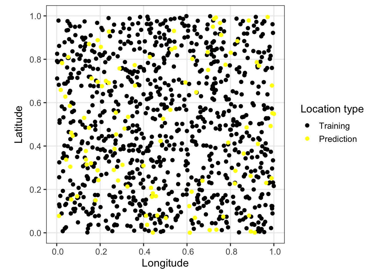
#| fig-cap: "Plot of 900 training locations and 100 prediction locations."
# load packages
suppressMessages({
  library(nimble)
  library(BayesNSGP)
  library(tidyverse)
  library(sf)
  library(coda)
  library(MCMCvis)
})
N <- 900 # training locations
P <- 100 # prediction plocations
M <- N+P # Total number of locations

set.seed(1)

# Simulate data
coords = matrix( 0, M, 2 )
coords[,1] = runif(M,0,1)
coords[,2] = runif(M,0, 1)

coords <- data.frame(x = coords[, 1], y = coords[, 2], id = 1:M)
coords$type <- c(rep("N", N), rep("P", P))
# the first N locations are training and the rest are prediction locations

# Coordinates for plotting
coords.sf <- st_as_sf(coords,
                      coords = c('x', 'y'))
ggplot() +
  geom_sf(data = coords.sf,
          aes(color = type),
          size = 2 ) +
  scale_color_manual(
    values = c("N" = "black", "P" = "yellow"),
    labels = c("Training", "Prediction")) +
  theme_bw(base_size = 14) +
  labs(
    x = "Longitude",
    y = "Latitude",
    color = "Location type"
  )
```
Before building our neighbor sets, a crucial requirement of Vecchia’s approximation is that the spatial locations must be ordered along a specific coordinate axis. This ordering guarantees that the graph structure remains directed and acyclic (a DAG), preventing circular conditioning loops.
We use the `computeNeighbors()` function to process our raw coordinates. This function sorts the rows along the horizontal axis (e.g., longitude/easting). Once sorted, it iterates through each location $i$ and searches exclusively among its preceding neighbors $(j<i)$ to find the $k=15$ nearest points based on Euclidean distance. For the first $k$ locations in the dataset, the conditioning set naturally defaults to all available predecessors $(i−1)$.
```{r}
#| label: NNGP_setup
#| cache: FALSE
k = 15 # number of nearest neighbors

# Sort coordinates and find the k nearest historical neighbors for each node
Neighbors_full = computeNeighbors(coords, k)
str(Neighbors_full)
```
`computeNeighbors()` produces several structures that are required to simulate the spatial random effects $\boldsymbol\omega$ and for model fitting in the NIMBLE model:
- `coords_sorted`: The matrix of coordinates, reordered sequentially by their horizontal positions.
- `edist_sorted`: Matrix ($M \times M$) of pairwise distances between sorted coordinates
- `neighbors`: Binary matrix $(M\times M)$ indicating neighbor relationships
- `neighbor_idx`: Matrix ($M\times K$) where row $i$ lists the sorted row-indices of the 15 chosen neighbors for that location.
- `neighbors_dist`: Matrix ($M\times K$) matrix storing the euclidean distances from each node to its respective neighbors.
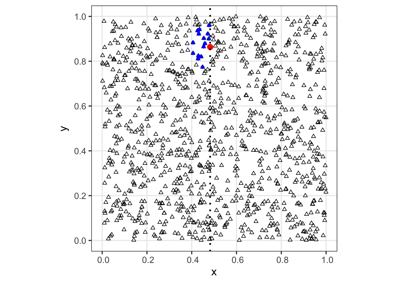
Using the `displayNeighbors()` function, we can visually inspect the DAG layout for the 500th location. The red triangle indicates the focal location, while the blue triangles represent its selected neighbors. Due to the ordering constraint, only locations that precede it in the sequence are eligible as neighbors. As a result, its candidate neighborhood is restricted on the right-hand side, and closer geometrically adjacent locations that appear later in the ordering (i.e., further along the horizontal gradient) cannot be selected.
```{r}
#| label: displayNeighbors
#| fig-cap: "Plot of neighbor set for a given location based on an ordered Nearest-Neighbor Gaussian Process (NNGP) constructed using Vecchia's approximation."
# Visualize the neighbor graph structure for a specific node
displayNeighbors(ind = 500, coords.sorted = Neighbors_full$coords_sorted, neighbor_idx = Neighbors_full$neighbor_idx)
```
## 3.2 The Direct Acyclic Weight Matrices ($A$ and $D$)
Once the neighbor topological graph is constructed, the spatial process can be parameterized using the sparse structural matrices $\boldsymbol{A}$ and $\boldsymbol{D}$. As introduced in Section 1.2.1, the NNGP decomposes a dense spatial process into a sequence of local linear regressions:
$$\omega(s_i) = \sum_{j \in S(s_i)} A_{ij} \omega(s_j) + \epsilon_i, \quad \epsilon_i \sim \mathcal{N}(0, D_{ii})$$
where: $\boldsymbol{A}$ acts as a spatial weight matrix, storing the regression coefficients $A_{ij}$ that dictate how much information $\omega(s_i)$ inherits from its conditioning neighbors. $\boldsymbol{D}$ acts as a local conditional variance matrix, where the diagonal element $D_{ii}$ tracks the residual variance (the unexplained spatial variation) left over after conditioning on those $k$ neighbors.
By calculating these parameters locally for every location, we can evaluate the joint spatial likelihood or construct the precision matrix without ever building or inverting a dense $M \times M$ matrix.
### 3.2.1 Computing $A$ and $D$ with `computeAD()`
To maximize efficiency, we do not want to construct or store the massive, mostly empty $M \times M$ sparse matrices $\boldsymbol{A}$ and $\boldsymbol{D}$ in memory. Instead, our package function `computeAD()` automates the local kriging calculations and packs the non-zero coefficients into a highly compressed, dense $M \times (k+1)$ matrix matrix layout.
For a specified length scale ($\rho$) and process variance ($\sigma^2$), the rows of this matrix map out as follows:
| Row index ($i$) | Columns $1$ to $k$ | Column $k+1$ |
|:-----------------------|:-----------------------|:-----------------------|
| **Location** $1$ | Neighbor Weights ($A_{1, j \in S(s_1)}$) | Conditional Variance ($D_{11}$) |
| **Location** $2$ | Neighbor Weights ($A_{2, j \in S(s_2)}$) | Conditional Variance ($D_{22}$) |
| **Location** $M$ | Neighbor Weights ($A_{M, j \in S(s_M)}$) | Conditional Variance ($D_{MM}$) |
: The first $k$ columns store the active neighbor weights from the matrix $A$, while the $(k+1)$-th column stores the diagonal elements of $\boldsymbol{D}$.
```{r}
#| label: ADcompute
# Define true exponential covariance parameter values
rho = 0.1
sigma2 = 0.3

# Compute local regression weights and conditional variances
AD_full <- computeAD(Neighbors_full$edist_sorted, Neighbors_full$neighbors_dist, Neighbors_full$neighbor_idx, rho, sigma2, k )

# Inspect dimensions of the resulting payload
dim(AD_full)
```
The returned object `AD_full` contains exactly $M = 1000$ rows and $k+1 = 16$ columns. By mapping out these local structural values directly, this approach eliminates the need for expensive $\mathcal{O}(M^3)$ global matrix operations during MCMC execution. Instead, it breaks the spatial process down into a series of highly localized, independent calculations, enabling seamless scalability when we embed the process into NIMBLE.
## 3.3 **Efficient Simulation from an NNGP Model**
With our neighborhood topology (`Neighbors_full`) and sparse weight structures (`AD_full`) established, we can now simulate the latent spatial process.
In a traditional Gaussian process framework, simulating a realization $\boldsymbol{\omega}$ at $M = 1000$ locations requires computing the Cholesky factorization of the dense $M \times M$ covariance matrix $\boldsymbol{K}$, a step that scales as $\mathcal{O}(M^3)$. The NNGP bypasses this bottleneck by leveraging the directed acyclic graph (DAG) structure. As described by @datta2022nearest, we can simulate $\boldsymbol{\omega}$ sequentially following its directional ordering:
$$\omega(s_1) \sim \mathcal{N}(0, D_{11})$$ $$\omega(s_i) = \sum_{j \in S(s_i)} A_{ij} \omega(s_j) + \epsilon_i, \quad \epsilon_i \sim \mathcal{N}(0, D_{ii}) \quad \text{for } i = 2, \ldots, M$$
Because each location only requires a linear combination of its $k$ pre-calculated neighbors plus a univariate normal draw, the entire spatial field can be simulated in a highly efficient $\mathcal{O}(Mk)$ operations. BayesNSGP's function `rmnorn_NN_GP` preforms this fast sequential update.
```{r}
#| label: sim_data
#| cache: FALSE
# Simulate the latent spatial random effects (omega)
omega <-  rmnorm_NN_GP(n = 1, mu = rep(0, M), AD = AD_full[1:M, 1:(k+1)], neighbors.id = Neighbors_full$neighbor_idx[1:M, 1:k])

# Simulate Poisson counts using a log-link
mu0 <- log(20)
lambda <- exp(mu0 + omega)
y <- rpois(M, lambda)

# Preview the simulated dataset
head(y)
```
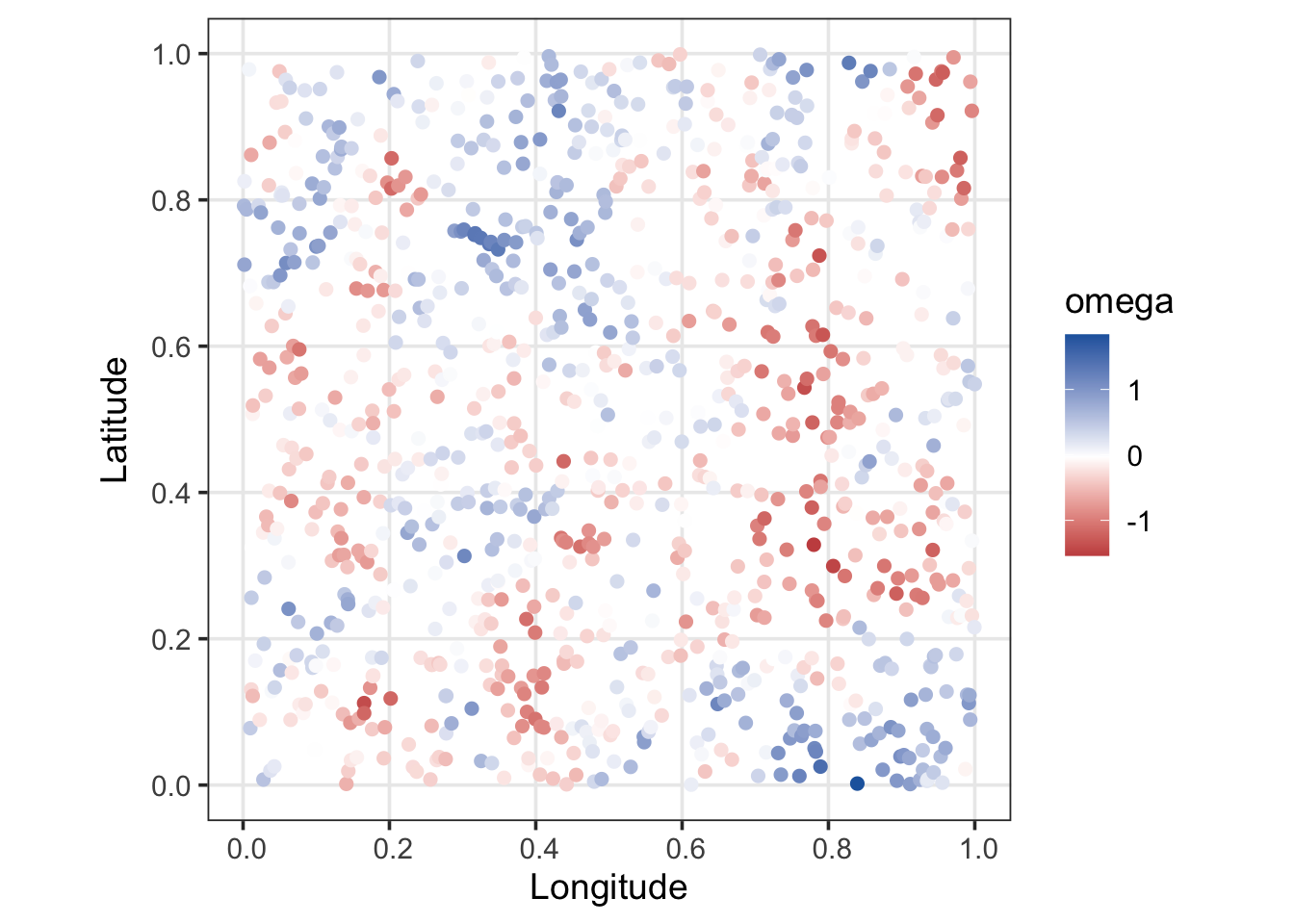
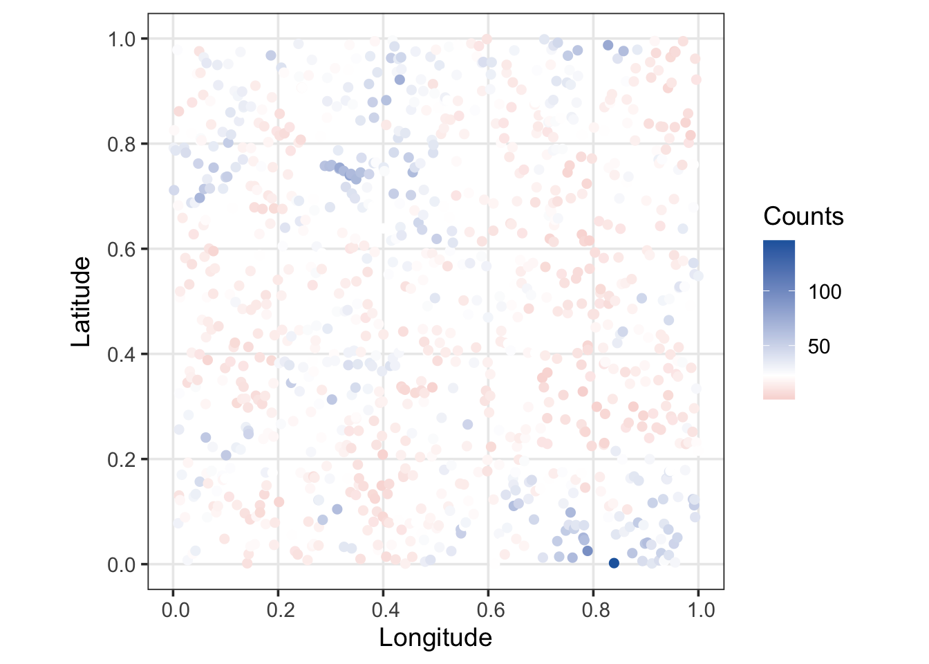
### 3.3.1 Visualizing the Spatial Surface
To verify that the NNGP successfully captures the intended spatial structure across our region, we project the simulated spatial field $(\boldsymbol\omega)$ and counts $(y)$ onto maps.
```{r}
#| label: plot_omega
#| fig-cap: "Simulated spatial field (omega) across the study region."
# Organise into a structured data frame for visualization
y.df <- data.frame(x = Neighbors_full$coords_sorted[, 1],
                   y =  Neighbors_full$coords_sorted[, 2],
                   counts = y,
                   omega = omega,
                   type = Neighbors_full$coords_sorted[, "type"],
                   id = Neighbors_full$coords_sorted[,3])

y.sf <- st_as_sf(y.df, coords = c('x', 'y'))

ggplot() +
  geom_sf(data = y.sf , aes(col = omega),  size = 2) +
  theme_bw(base_size = 14) +
  scale_color_gradient2(midpoint = mean(y.df$omega), low = '#B2182B', mid = 'white', high = '#2166AC',
                        na.value = NA) +
  labs(x = 'Longitude', y = 'Latitude', col = 'omega')
```
```{r}
#| label: plot_simulated_counts
#| fig-cap: "Simulated Poisson counts across the study region, showing distinct patterns of spatial autocorrelation."
ggplot() +
  geom_sf(data = y.sf , aes(col = counts),  size = 2) +
  theme_bw(base_size = 14) +
  scale_color_gradient2(midpoint = mean(y.df$counts), low = '#B2182B', mid = 'white', high = '#2166AC',
                        na.value = NA) +
  labs(x = 'Longitude', y = 'Latitude', col = 'Counts')
```
# 4. NIMBLE Model Fitting
With our simulated data ready, we can now fit the spatial Poisson GLM using the 900 training locations ($N$). Because our out-of-sample prediction testing set ($P$) was randomly interspersed among the original coordinates, dropping them to form the training set requires us to rebuild a dedicated neighbor graph exclusively for the training coordinates.
## 4.1 Subsetting the Training Data
When we re-run `computeNeighbors()` on the training coordinates, the function will sort the locations along the horizontal axis. Because this changes the row order of our training coordinates, we must be careful to map our response vector `y` using the newly sorted location IDs. This ensures that the counts $y_i$ perfectly align with the spatial random effects $\omega_i$.
```{r}
#| label: subset_train
# 1. Isolate raw training coordinates from the globally simulated data
coords.train.raw <- Neighbors_full$coords_sorted[Neighbors_full$coords_sorted$type == "N", c("x", "y", "id")]

# 2. Re-compute a dedicated neighbor topology for training ONLY
Neighbors_train <- computeNeighbors(coords.train.raw, k)

# Extract graph parameters
coords.sorted.train <- Neighbors_train$coords_sorted[, 1:2]
edist.sorted.train  <- Neighbors_train$edist_sorted
nid.dist.train      <- Neighbors_train$neighbors_dist
neighbors.id.train  <- Neighbors_train$neighbor_idx

# 3. CRITICAL: Match counts to the newly sorted training graph row order using unique IDs
sorted_train_ids <- Neighbors_train$coords_sorted$id
y.train <- y.df$counts[match(sorted_train_ids, y.df$id)]
```
## 4.2 Building the BUGS Code
We define our model structure using NIMBLE's `nimbleCode` function. Note how our package's custom `computeAD()` function and `dmnorm_NN_GP()` distribution are embedded directly within the BUGS code chunk. This allows NIMBLE to dynamically update the neighborhood weights whenever the spatial parameters $\rho$ or $\sigma^2$ change during MCMC execution.
```{r}
#| label: nimble_model
#| eval: TRUE
# Package data into a structured list for NIMBLE constants
win.data <- list(
  N = N,
  mu = rep(0, N),
  edist = edist.sorted.train,
  dmax = max(edist.sorted.train),
  dmin = min(edist.sorted.train[edist.sorted.train != 0]),
  nid.dist = nid.dist.train,
  n.id = neighbors.id.train,
  k = k
)

# Define the BUGS model structure
Mtest <- nimbleCode({

  # Priors
  mu0 ~ dnorm(0, sd = 2)
  sigma2 ~ dinvgamma(3, 1)
  rho ~ dunif(dmin/3, dmax/3)

  # NNGP Joint Density construction
  AD[1:N, 1:(k+1)] <- computeAD(edist[1:N, 1:N], nid.dist[1:N, 1:(k+1)], n.id[1:N, 1:k], rho, sigma2, k)
  omega[1:N] ~ dmnorm_NN_GP(mu[1:N], AD[1:N, 1:(k+1)], n.id[1:N, 1:k])

  # Soft sum-to-zero constraint for intercept identifiability
  constraint ~ dnorm(sum(omega[1:N]), sd = 1)

  # Likelihood loop
  for (i in 1:N) {
    log(lambda[i]) <- mu0 + omega[i]
    y[i] ~ dpois(lambda[i])
  }
})
```
### 4.2.1 Using `dmnorm_NN_GP()` in Practice
The core mathematical engine of this package inside the BUGS framework is the custom vector distribution `dmnorm_NN_GP(mu, AD, n.id)`. In standard NIMBLE, a typical spatial process might be declared using `dmnorm(mu, cov = K)` or `dmnorm(mu, prec = Q)`. However, passing a dense $M \times M$ matrix forces NIMBLE's C++ backend to execute an $\mathcal{O}(M^3)$ Cholesky factorization every time a hyperparameter shifts.
Our `dmnorm_NN_GP()` distribution side-steps this completely by operating directly on the local DAG parameters. It takes three essential arguments:
1. `mu[1:N]`: The mean vector for the spatial process (here, a vector of zeros).
2. `AD[1:N, 1:(k+1)]`: The dynamically updated matrix containing the local regression weights $A$ in the first $k$ columns and the conditional variances $D$ in the final column. Calculated from `computeAD`
3. `n.id[1:N, 1:k]`: The static integer matrix mapping the neighbor indices for every location. Generated by `computeNeighbors()`.
By utilizing this distribution, NIMBLE automatically handles the complex conditional independence structures of the NNGP behind the scenes. This allows you to treat the large-scale spatial process just like any other standard multivariate distribution in your hierarchical model, while enjoying massive improvements in runtime speed and memory savings.
We also introduce a soft sum-to-zero constraint (`constraint ~ dnorm(sum(omega[1:N]), sd = 1)`) on the spatial field. Because both the intercept $\mu_0$ and the spatial random effect $\boldsymbol{\omega}$ modify the mean log-intensity, adding this constraint prevents them from shifting together, drastically improving parameter identifiability and MCMC mixing.
### 4.2.1 Model initialization
Before running the MCMC, we initialize the model parameters. To provide a realistic starting point for the spatial field, we initialize $\boldsymbol{\omega}$ by using `rmnorm_NN_GP`
```{r}
#| label: initialize_model
# Establish initial values for hyperparameters
GP.inits <- list(rho = mean(edist.sorted.train)/3, sigma2 = 1)

# Spatial field initial value s
omega.inits <-  rmnorm_NN_GP(n = 1, mu = rep(0, N), AD = computeAD(edist.sorted.train, nid.dist.train, neighbors.id.train, GP.inits$rho, GP.inits$sigma2, k  )  , neighbors.id = Neighbors_full$neighbor_idx[1:M, 1:k])


# Generate realistic initial values for spatial random effects
inits <- list(
  omega = omega.inits ,
  mu0 = rnorm(1),
  rho = GP.inits$rho,
  sigma2 = GP.inits$sigma2
)

# Build the uncompiled NIMBLE model object
Model <- nimbleModel(
  code = Mtest,
  data = list(y = y.train, constraint = 0),
  constants = win.data,
  inits = inits,
  calculate = TRUE
)
```
### 4.2.2 Model diagnostics
A key best-practice when writing custom NIMBLE components is checking that the uncompiled log-likelihood values calculate successfully without producing any structural missing values (`NaN`) or infinite values `-Inf`.
We test our package's custom backend by explicitly evaluating the joint NNGP probability log-density, followed by a global calculation of the complete model network.
```{r}
#| label: diagnostic_check
# Verify the custom NNGP probability density evaluates correctly
Model$calculate("omega")
# Evaluate the total model network log-density
Model$calculate()
```
If `Model$calculate()` returns a valid, finite numeric scalar (the sum of log-densities across all nodes), it serves as a robust indication that your graph architecture is completely and correctly specified, parameters match their data nodes, and the model is fully prepared for compilation and sampling.
# 5. MCMC Configuration and Sampler Comparison
To demonstrate the advantages of our optimized package architecture, we will configure and compare three distinct MCMC samplers for the spatial field $\boldsymbol{\omega}$:
1. **Random walk block sampler (`RW_block`)**: NIMBLE's default configuration for multivariate normal distributions. This joint sampler updates the entire vector $\boldsymbol{\omega}$ simultaneously as a single correlated block.
2. **Individual random walk sampler (`RW`)**: A non-default configuration where we override NIMBLE to assign an independent, standard scalar Random Walk sampler to each individual element $\omega_i$.
3. **NNGP-Specific Random Walk Metropolis-Hastings Sampler (`RW_NN_GP`)**: `BayesNSGP`'s custom single-node sampler . It updates each element $\omega_i$ individually, but exploits the local DAG neighborhood structure to bypass the global model density entirely. By evaluating changes only within an item's immediate local neighborhood, it performs updates in linear time—offering significantly improved execution speed while targeting the exact same mathematical posterior.
## 5.1 Random walk block sampler `(RWblock)`
We begin by evaluating NIMBLE's default configuration. Because `omega` is defined as a multivariate vector under the `dmnorm_NN_GP` distribution, NIMBLE automatically assigns an `RW_block` sampler to the entire spatial field.
```{r}
#| label: default_RWblock
#| eval: TRUE
#| cache: TRUE
# Configure the default MCMC structure
Modelconf = configureMCMC(Model)
Modelconf$addMonitors("omega")
```
```{r}
#| eval: FALSE
# Build and compile the model components
Modelmcmc = buildMCMC(Modelconf)
cModel <- compileNimble(Model)
Modelmod = compileNimble(Modelmcmc, project = Model, resetFunctions = TRUE)

# Run the MCMC chains and benchmark execution time
RWblock_time  <- system.time(Modelmcmc.out.RWblock <- runMCMC(Modelmod,niter = 10000, nburnin = 5000,thin = 5, nchains = 2,  samplesAsCodaMCMC = TRUE, summary = TRUE))
```
```{r echo = FALSE, eval = FALSE}
## save the output of the (long) MCMC run.
## this does *not* get executed by default, but only manually, when you do the MCMC run again
save('Modelmcmc.out.RWblock', 'RWblock_time', file = '../cache/RWblock_sampler.RData')
```
```{r echo = FALSE}
## now load in the output of the run
## this gets executed every time the example is built
load('../cache/RWblock_sampler.RData')
```
```{r}
#| label: RWblock_post
# Extract MCMC samples
samples.RWblock <- Modelmcmc.out.RWblock$samples

# Review hyperparameter summaries
MCMCsummary(samples.RWblock[, c("mu0", "rho", "sigma2")]) # Clearly convergence and mixing not good.
mu0; rho; sigma2
```
### 5.1.2 MCMC diagnostics
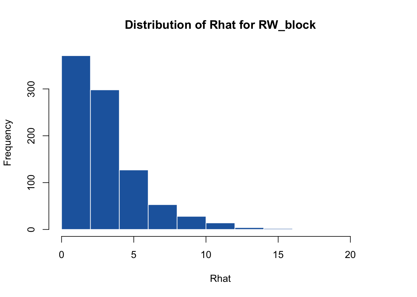
To evaluate how well the spatial field converged under the default blocking scheme, we extract the summaries for all $N= 900$ elements of $\boldsymbol{\omega}$ and calculate the proportion of nodes that failed to converge $(R \geq 1.2)$.
```{r}
#| label: default_diagnostics
# Extract summaries for the spatial field elements
omega.post.RWblock <- MCMCvis::MCMCsummary(samples.RWblock, params = "omega")
head(omega.post.RWblock)
# Check distribution of Gelman-Rubin diagnostic (Rhat)
hist(omega.post.RWblock$Rhat, main = "Distribution of Rhat for RW_block", xlab = "Rhat",
     col = "#2166AC",
     border = "white")
# Calculate the proportion of non-converged spatial terms
non_converged_prop <- sum(omega.post.RWblock$Rhat > 1.2) / N
non_converged_prop
```
About 85% of the spatial locations fail to converge. This poor behavior occurs because the massive block proposal is highly inefficient; proposing updates to 900 dimensions at once leads to extremely low acceptance rates.
### 5.1.3 **MCMC efficiency**
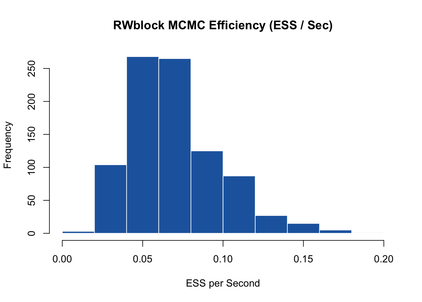
Finally, we calculate the **MCMC efficiency** (Effective Sample Size per second of runtime) for the spatial field to establish our baseline benchmark.
```{r}
#| label: default_efficiency
# Calculate effective sample size per second of elapsed wall-clock time
RWblock.MCMCeff <- omega.post.RWblock$n.eff / RWblock_time[3]

# Visualize sampling efficiency across the field
hist(RWblock.MCMCeff, main = "RWblock MCMC Efficiency (ESS / Sec)", xlab = "ESS per Second",
     col = "#2166AC",
     border = "white")
```
## 5.2 Individual Random walk `(RW)`
To address the high-dimensional bottleneck of updating the entire spatial field at once, we can override NIMBLE's default behavior. In this configuration, we remove the joint block sampler and assign independent, standard single-node Random Walk (`RW`) samplers to each individual element $\omega_i$.
While breaking the spatial field into 900 separate scalar samplers increases the number of update steps per iteration, it avoids the massive rejection rate of the high-dimensional block proposal, allowing the chains to traverse the target distribution much more freely.
```{r}
#| label: idRW
#| eval: TRUE
#| cache: TRUE
# Configure a new MCMC object
Modelconf = configureMCMC(Model)
Modelconf$addMonitors("omega")
# Remove the default joint multivariate block sampler for omega
Modelconf$removeSamplers("omega")

# Assign an independent scalar RW sampler to each individual spatial node
for (i in 1:N) {
  Modelconf$addSampler(target = paste0("omega[", i, "]"), type = "RW")
}

# Inspect the updated sampler configurations
Modelconf
```
```{r, eval=FALSE}
# Build and compile the modified model
Modelmcmc = buildMCMC(Modelconf)
cModel <- compileNimble(Model)
Modelmod = compileNimble(Modelmcmc, project = Model, resetFunctions = TRUE)

# Run the MCMC chains and benchmark execution time
RW_time  <- system.time(Modelmcmc.out.RW <- runMCMC(Modelmod,niter = 10000, nburnin = 5000,thin = 5, nchains = 2,  samplesAsCodaMCMC = TRUE, summary = TRUE))
```
```{r echo = FALSE, eval = FALSE}
## save the output of the (long) MCMC run.
## this does *not* get executed by default, but only manually, when you do the MCMC run again
saveRDS(
list(
samples = Modelmcmc.out.RW,
runtime = RW_time
),
"../cache/RW_sampler.rds"
)
```
```{r echo = FALSE}
## now load in the output of the run
## this gets executed every time the example is built
out <- readRDS("../cache/RW_sampler.rds")
Modelmcmc.out.RW <- out$samples
RW_time <- out$runtime
```
```{r}
#| label: RW_post
# Extract MCMC samples
samples.RWid <- Modelmcmc.out.RW$samples

# Review hyperparameter summaries
MCMCsummary(samples.RWid[, c("mu0", "rho", "sigma2")])
mu0; rho; sigma2
```
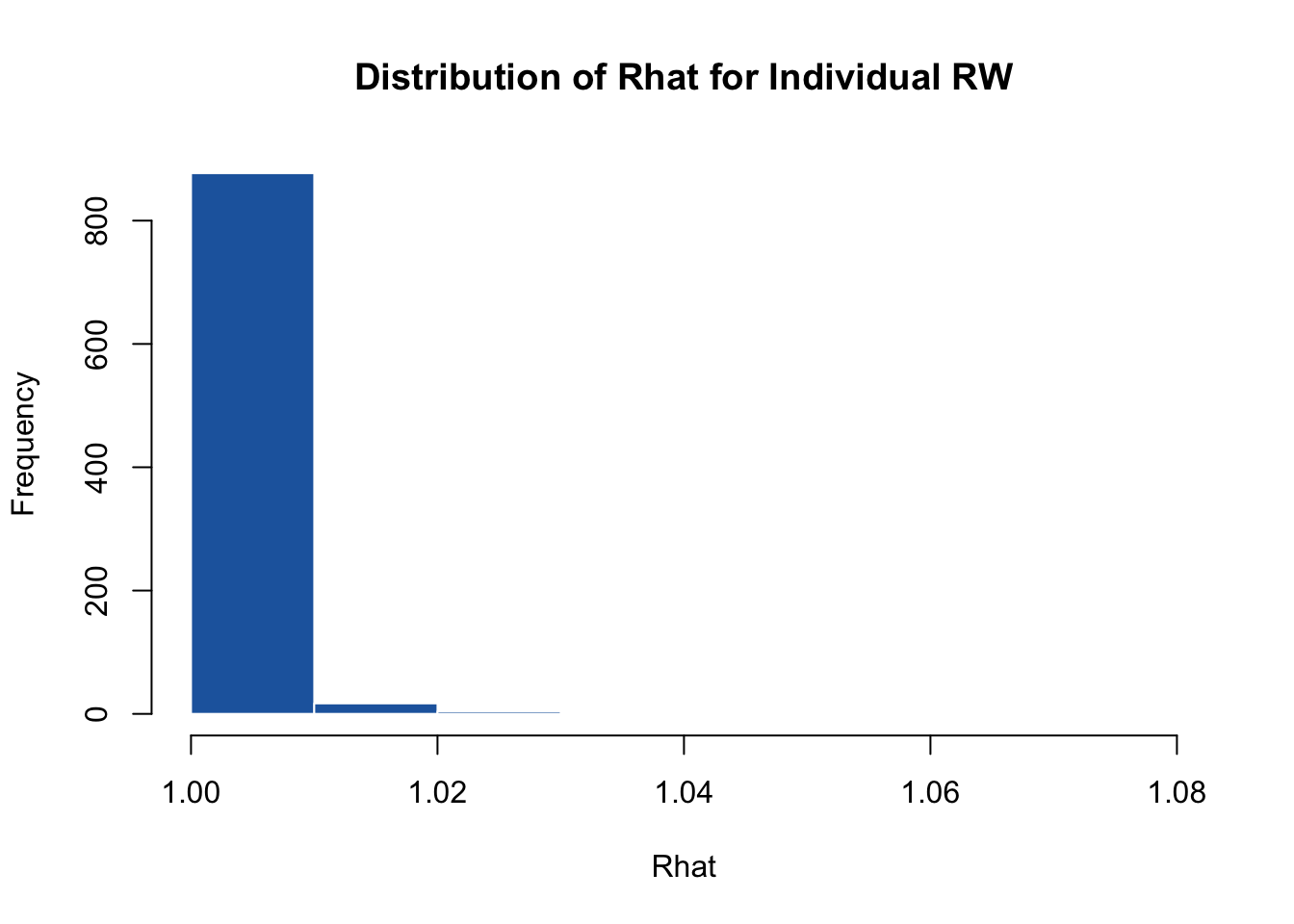
### 5.2.2 MCMC diagnostics
We isolate the posterior summaries for the spatial field elements to examine how switching to single-node updates affects model convergence $\hat{R}$ .
```{r}
#| label: idRW_diagnostics
# Extract spatial field summaries
omega.post.RWid <- MCMCvis::MCMCsummary(samples.RWid, params = "omega")
head(omega.post.RWid)
# Visualize the distribution of Rhat values
hist(omega.post.RWid$Rhat, main = "Distribution of Rhat for Individual RW", xlab = "Rhat",
     col = "#2166AC",
     border = "white")
# Calculate the proportion of non-converged spatial terms
sum(omega.post.RWid$Rhat > 1.2) / N
```
Using individual `RW`samplers, we see a dramatic improvement in convergence and mixing across the spatial parameters. All nodes converge compared to the default blocking scheme.
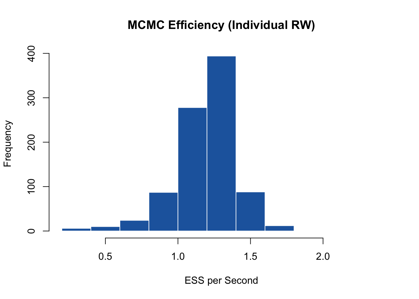
### 5.2.3 **MCMC efficiency**
```{r}
#| label: idRW_efficiency
# Calculate effective sample size per second for the individual samplers
RWid.MCMCeff <- omega.post.RWid$n.eff / RW_time[3]
hist(RWid.MCMCeff, main = "MCMC Efficiency (Individual RW)", xlab = "ESS per Second",
     col = "#2166AC",
     border = "white")
# Calculate the runtime ratio between individual RW and RW_block
(RW_time[3] ) / (RWblock_time[3])
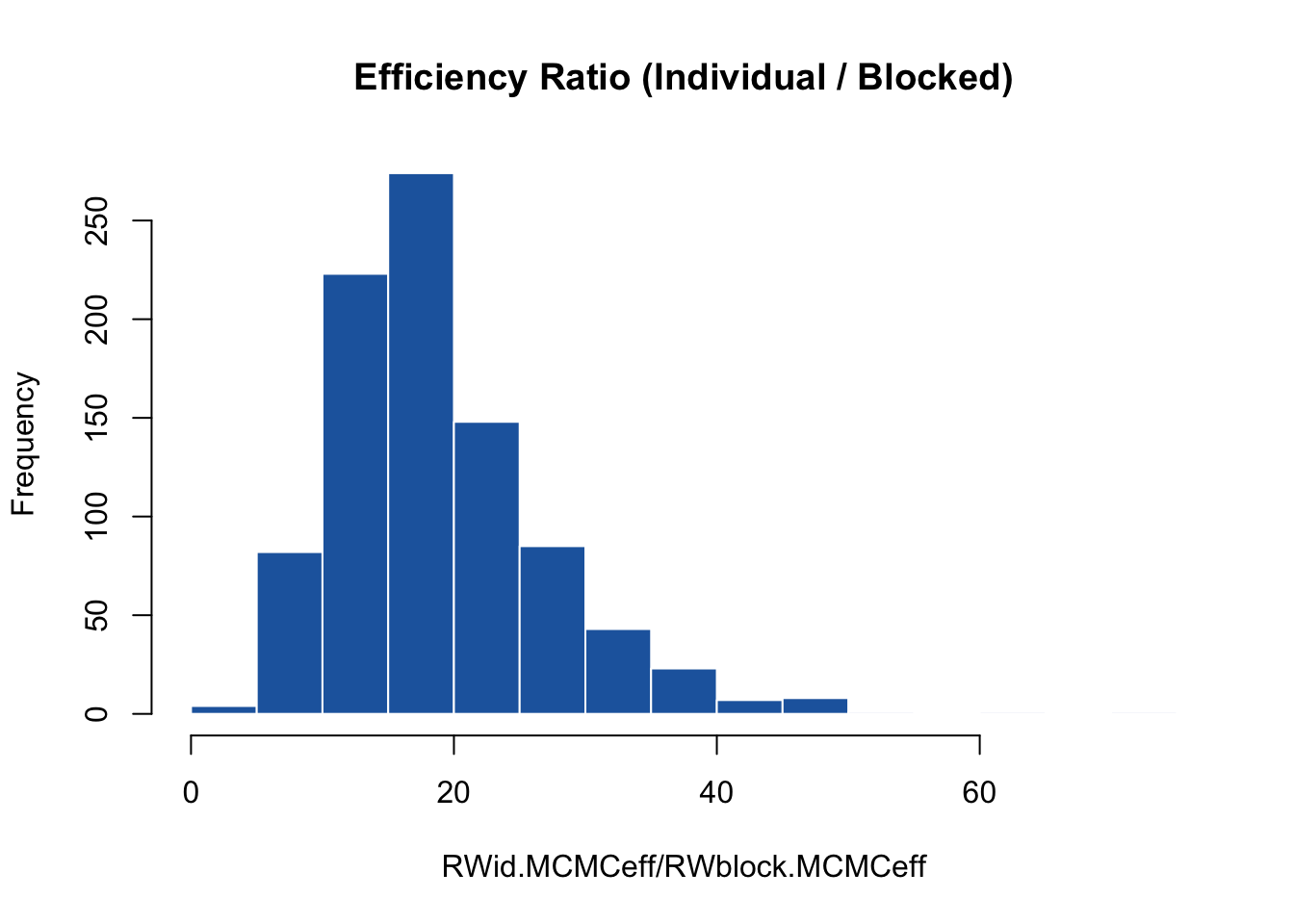
# Compare efficiency distribution and extract the median gain
hist(RWid.MCMCeff / RWblock.MCMCeff, main = "Efficiency Ratio (Individual / Blocked)",
     col = "#2166AC",
     border = "white")
median(RWid.MCMCeff / RWblock.MCMCeff)
```
#### Why the Individual Sampler Wins
The benchmark numbers reveal an important MCMC paradox: even though the individual `RW` configuration is roughly **7.5 times slower** in absolute wall-clock time, it is approximately **18 times more efficient** than the default `RW_block` sampler.
The block sampler scales poorly because evaluating a 900-dimensional proposal forces an all-or-nothing outcome; if a single coordinate is rejected, the entire block is thrown out, leading to stagnant chains. Independent scalar updates take longer to execute mechanically, but their drastically higher proposal acceptance rates yield vastly more uncorrelated posterior samples per second.
### 5.2.4 Relative Bias
Finally, we calculate the median relative bias $(RB)$ across our training nodes to ensure that our point estimates are successfully reconstructing the true underlying spatial field $\omega_{train}$ that we simulated.
```{r}
#| label: idRW_bias
# Extract the true spatial random effects used during data simulation
omega.train <- omega[y.df$type=="N"]

# Calculate relative bias for each node
rb.idRW <- (omega.post.RWid$mean - omega.train) / omega.train
median(rb.idRW)
```
## 5.3 NNGP-Specific Random Walk Metropolis-Hastings Sampler `(RW_NN_GP)`
`BayesNSGP`'s custom single-node sampler, `RW_NN_GP`, delivers the best of both worlds. Like the individual `RW` configuration, it updates each spatial random effect $\omega_i$ individually to maintain high proposal acceptance rates. However, instead of evaluating the full model density at every single step, it utilizes a localized "reverse-neighbor" lookup graph behind the scenes.
When updating an individual node $\omega_i$, the `RW_NN_GP` sampler only calculates the density changes for that specific node and its immediate directed "children" (the downstream nodes that condition upon it) in the Directed Acyclic Graph (DAG). This cuts the computational cost of an individual node update down to a trivial $\mathcal{O}(k^2)$ operations. As a result, the execution time per MCMC iteration becomes incredibly fast and completely independent of the total number of spatial locations $M$.
```{r}
#| label: RW_NNGP
#| eval: TRUE
# Configure a new MCMC object
Modelconf = configureMCMC(Model)
Modelconf$addMonitors("omega")
# Remove the default joint multivariate block sampler
Modelconf$removeSamplers("omega")

# Assign our optimized custom local NNGP sampler to each node
for (i in 1:N) {
  Modelconf$addSampler(target = paste0("omega[", i, "]"), type = "RW_NN_GP", control = list(AD = "AD", neighbors.id = neighbors.id.train))
}

# Verify the customized sampler list configuration
Modelconf
```
```{r}
#| eval: FALSE
# Build and compile the optimized model components
Modelmcmc = buildMCMC(Modelconf)
cModel <- compileNimble(Model)
Modelmod = compileNimble(Modelmcmc, project = Model, resetFunctions = TRUE)

# Run the MCMC chains and benchmark execution time
RWNNGP_time  <- system.time(Modelmcmc.out.RWNNGP <- runMCMC(Modelmod,niter = 10000, nburnin = 5000,thin = 5, nchains = 2,  samplesAsCodaMCMC = TRUE, summary = TRUE))
```
```{r echo = FALSE, eval=FALSE}
## save the output of the (long) MCMC run.
## this does *not* get executed by default, but only manually, when you do the MCMC run again
saveRDS(
list(
samples = Modelmcmc.out.RWNNGP,
runtime = RWNNGP_time
),
"../cache/RWNNGP_sampler.rds"
)
```
```{r echo=FALSE}
## now load in the output of the run
## this gets executed every time the example is built
out.RWNNGP <- readRDS("../cache/RWNNGP_sampler.rds")
Modelmcmc.out.RWNNGP <- out.RWNNGP$samples
RWNNGP_time <- out.RWNNGP$runtime
```
```{r}
#| label: RWNNGP_post
# Extract MCMC samples
samples.RWNNGP <- Modelmcmc.out.RWNNGP$samples

# Review hyperparameter summaries
MCMCsummary(samples.RWNNGP[, c("mu0", "rho", "sigma2")])
mu0; rho; sigma2
```
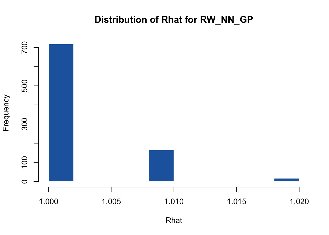
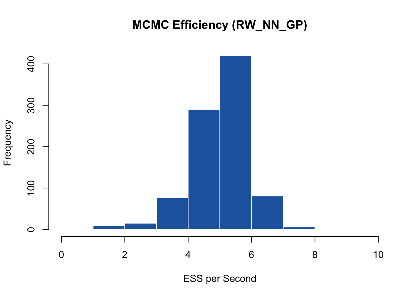
### 5.3.2 Analyzing Convergence and Efficiency Gains
We extract the posterior summaries for the spatial field elements under the `RW_NN_GP` configuration to evaluate convergence profiles and compute the sampling efficiency.
```{r}
#| label: RW_NNGP_diagnostics
# Extract spatial field summaries
omega.post.RWNNGP <- MCMCvis::MCMCsummary(samples.RWNNGP, params = "omega")
head(omega.post.RWNNGP)
# Visualize the distribution of Rhat values
hist(omega.post.RWNNGP$Rhat, main = "Distribution of Rhat for RW_NN_GP", xlab = "Rhat",
     col = "#2166AC",
     border = "white")
# Calculate the proportion of non-converged spatial terms
sum(omega.post.RWNNGP$Rhat > 1.2) / N
# Calculate effective sample size per second
RWNNGP.MCMCeff <- omega.post.RWNNGP$n.eff / RWNNGP_time[3]
hist(RWNNGP.MCMCeff, main = "MCMC Efficiency (RW_NN_GP)", xlab = "ESS per Second",
     col = "#2166AC",
     border = "white")
```
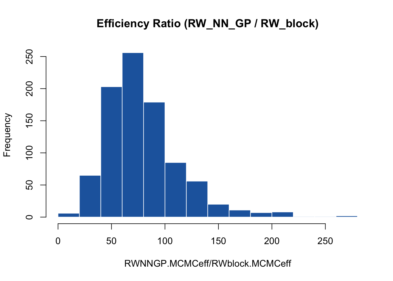
### 5.3.3 MCMC Efficiency Comparisons
To finalize our comparison, we directly contrast the sampling efficiency (ESS / Sec) of `RW_NN_GP` against both the default block sampler and the standard individual random walk sampler.
```{r}
#| label: efficiency_comparisons
# Relative efficiency compared to the default RW_block
hist(RWNNGP.MCMCeff / RWblock.MCMCeff, main = "Efficiency Ratio (RW_NN_GP / RW_block)",
     col = "#2166AC",
     border = "white")
median(RWNNGP.MCMCeff / RWblock.MCMCeff)
# Relative efficiency compared to the standard individual RW
hist(RWNNGP.MCMCeff / RWid.MCMCeff, main = "Efficiency Ratio (RW_NN_GP / Individual RW)",
     col = "#2166AC",
     border = "white")
median(RWNNGP.MCMCeff / RWid.MCMCeff)
```
The results highlight the massive practical utility of `RW_NN_GP`. By combining the mixing properties of single-node updates with highly optimized localized likelihood evaluations, the `RW_NN_GP` sampler is approximately **4 times more efficient** than the standard individual `RW` sampler, and orders of magnitude more efficient than the default blocking method.
**Note on Scalability:** Because the local evaluation cost of `RW_NN_GP` depends strictly on the neighbor size $k$ rather than the data size $M$, this efficiency advantage will grow exponentially as the number of spatial locations increases.
### 5.3.4 Validation of Posterior Means
As a final verification check, we compare the median relative bias $(RB)$ of the estimated random effects under both single-node sampling configurations to confirm that our custom local likelihood sampler accurately preserves the true posterior distribution.
```{r}
#| label: relative_bias_check
# Calculate relative bias for the custom NNGP sampler
rb.NNGP <- (omega.post.RWNNGP$mean - omega.train) / omega.train

# Contrast the median relative bias values
median(rb.NNGP)
median(rb.idRW)
```
The near-identical bias metrics confirm that `RW_NN_GP` targets the exact same mathematical posterior distribution as standard implementations, granting you identical statistical inference at a fraction of the computational runtime.
## 5.3.5 Summary of Results
To provide a clear picture of the performance trade-offs across the three sampling strategies, we evaluate them across three primary dimensions: absolute wall-clock runtime, mixing quality (measured by the proportion of parameters that successfully converged with $\hat{R} \le 1.2$), and overall MCMC efficiency (the median Effective Sample Size achieved per second of execution time).
The performance metrics across our $N = 900$ training locations are summarized below:
| Sampling Strategy | Relative Runtime | Convergence Success ($\hat{R} \le 1.2$) | Median MCMC Efficiency (ESS / Sec) | Relative Efficiency Gain |
|:--------------|:-------------:|:-------------:|:-------------:|:-------------:|
| **1. Default `RW_block`** | **1x** (Fastest per step) | \~17% | Baseline | Baseline (1x) |
| **2. Individual `RW`** | \~7.7x Slower | \~100% | Higher | \~17x More Efficient |
| **3. Custom `RW_NN_GP`** | \~1.9x Slower | \~100% | **Highest** | **\~70x More Efficient** |
### Key Takeaways
- **RW_block: Fast but poor mixing**
The default block sampler has the lowest wall-clock runtime per iteration, but exhibits poor mixing in this high-dimensional setting. Jointly proposing updates to all 900 spatial random effects leads to low acceptance rates and poor exploration of the posterior distribution, with only approximately 17% of parameters achieving convergence $(\hat{R}\leq1.2)$.
- **RW: Improved mixing at substantial computational cost**
Updating the spatial random effects one location at a time substantially improves convergence, with nearly all parameters satisfying the convergence criterion. However, each scalar update still requires evaluation of the full joint model density, resulting in a large increase in overall runtime.
- **RW_NN_GP: Improved mixing with localized computations**
The custom RW_NN_GP sampler combines single-location updates with NNGP-specific local likelihood calculations. This approach retains the favorable convergence properties of scalar updates while substantially reducing the computational burden associated with evaluating the full spatial model. As a result, it achieves the highest ESS per second among the three samplers.
Overall, the `RW_NN_GP` sampler provides the most favorable balance between computational cost and sampling efficiency while targeting the same posterior distribution as the standard samplers. Because each update depends only on a fixed neighborhood of size $(k)$, rather than all locations, the computational advantages are expected to become increasingly pronounced as the size of the spatial dataset grows.
# 6. Predictions
Gaussian processes (GPs) provide an exceptionally powerful framework for out-of-sample prediction because the latent spatial process at unobserved test locations naturally inherits the joint multivariate normal dependency of the training architecture.
Importantly, GP predictions yield more than just a single point estimate—they provide a full posterior predictive distribution. This quantified uncertainty is highly spatial: prediction variance is generally much lower (higher confidence) for test locations nested close to existing training data points, and expands outwards as you move into data-sparse regions.
### 6.1 Kriging Theory vs. NNGP Sequential Composition
In a traditional Gaussian process framework, predicting the latent spatial random effects $\boldsymbol{\omega}_0$ at $P$ unobserved locations based on $N$ observed training effects $\boldsymbol{\omega}$ relies on partitioned multivariate normal conditioning:
$$\begin{bmatrix} \boldsymbol{\omega}\\ \boldsymbol{\omega}_0 \end{bmatrix} \sim \mathcal{N} \left( \begin{bmatrix} \boldsymbol{0}\\ \boldsymbol{0} \end{bmatrix}, \begin{bmatrix} \boldsymbol{K}(X,X) & \boldsymbol{K}(X,X_0)\\ \boldsymbol{K}(X_0,X) & \boldsymbol{K}(X_0,X_0) \end{bmatrix} \right)$$
Using standard conditional normal theory, the exact posterior predictive distribution is:
$$\boldsymbol{\omega}_0 \mid \boldsymbol{\omega} \sim \mathcal{N}\left( \boldsymbol{K}(X_0,X) \boldsymbol{K}(X,X)^{-1}\boldsymbol{\omega} , \,\, \boldsymbol{K}(X_0,X_0) - \boldsymbol{K}(X_0,X) \boldsymbol{K}(X,X)^{-1}\boldsymbol{K}(X,X_0) \right)$$
Evaluating these equations directly requires inverting the dense $N \times N$ matrix $\boldsymbol{K}(X,X)$, which introduces an $\mathcal{O}(N^3)$ computational bottleneck for large datasets.
To circumvent this, `BayesNSGP`'s `NNGP.pred()` function executes prediction by applying the same local conditioning rules used to build the training graph. This function automatically handles coordinate sorting, neighbor selection, and distance calculations internally following **Algorithm 2 of @finley_efficient_2019**. Instead of querying all $N$ training locations, it finds the $k$ nearest training neighbors for each prediction coordinate, evaluating the conditional mean and variance in a lightweight, localized fraction of the time.
Consequently, prediction scales as $(\mathcal{O}(Pk^3))$, making posterior spatial interpolation feasible even for datasets containing thousands or tens of thousands of locations.
### 6.2 Executing the Prediction Loop
We iterate through each of our $P = 100$ held-out prediction locations. For every location, we loop through the saved post-burnin MCMC samples to draw a realization of the latent spatial term, convert it to a Poisson intensity ($\lambda$), and generate an out-of-sample count prediction via `rpois()`.
```{r}
#| label: NNGP_predict
#| eval: FALSE
# 1. Isolate the out-of-sample prediction coordinates
coords.predict <- Neighbors_full$coords_sorted[y.df$type =="P",1:2]

# 2. Extract and format posterior samples into a matrix
samples <- mcmc(do.call(rbind, samples.RWNNGP))

# Initialize storage matrix for predictions (MCMC samples x Prediction Locations)
MCMC_nsamples = dim(samples)[1]
y.pred = matrix(0, nrow = MCMC_nsamples, P)


# 3. Predict sequentially across all testing locations
for (i in 1:P) {

  new_loc <- coords.predict[i,]

  for (mc in 1:MCMC_nsamples) {

    # Extract parameter values for the current MCMC iteration
    mc.mu0 = samples[mc,"mu0"]
    mc.rho = samples[mc,"rho"]
    mc.sigma2 = samples[mc, "sigma2"]

    # Extract the full spatial random effects vector for this iteration
    mc.omega = samples[mc, paste0("omega[",1:N,"]" )]

    # Fast conditional prediction via our package backend (Finley et al. 2019 Algorithm 2)
    omega.pred  <- NNGP.pred(x0 = new_loc,coords_sorted = coords.sorted.train,
                             rho = mc.rho, sigma2 = mc.sigma2,
                             w.x0.all = mc.omega, k = k)

    # Map back to the Poisson likelihood framework
    lambda.pred <- exp(mc.mu0 + omega.pred)
    y.pred[mc, i] <- rpois(1, lambda.pred)

  }


}
```
```{r echo = FALSE, eval = FALSE}
## save the output of the (long) NNGP.pred run.
## this does *not* get executed by default, but only manually, when you do the NNGP.pred run again
save('y.pred', file = '../cache/nngp_pred.RData')
```
```{r echo = FALSE}
## now load in the output of the run
## this gets executed every time the example is built
load('../cache/nngp_pred.RData')
```
### 6.3 Predictive Accuracy Validation
To evaluate how accurately our spatial model reconstructs unobserved ecological counts, we extract the true generated counts for our test points and plot the distribution of the relative bias $(RB)$.
```{r}
#| label: prediction_bias
# Isolate the true, simulated counts for the testing locations
y.pred.true <- y.df$counts[y.df$type == "P"]

# Calculate posterior predictive summaries
y.pred.mean <- colMeans(y.pred)
y.pred.sd <- apply(y.pred, 2, sd)

# Calculate out-of-sample relative bias
rb.pred <- (y.pred.mean - y.pred.true) / y.pred.true

# Plot the bias distribution
hist(
  rb.pred,
  breaks = 10,
  main = "Out-of-Sample Prediction Relative Bias",
  xlab = "Relative Bias",
  col = "#2166AC",
  border = "white"
)
# Extract the median relative bias
median(rb.pred)
```
A median relative bias close to zero demonstrates that the NNGP local approximation successfully captures the continuous spatial process, enabling highly accurate, unbiased ecological forecasts at unobserved locations across your study region.
# 7. Conclusion
In this vignette, we demonstrated how to construct, fit, and predict from a Nearest-Neighbor Gaussian Process (NNGP) model in `NIMBLE` using `BayesNSGP`. By replacing dense covariance calculations with sparse local neighborhood operations, NNGPs provide a computationally efficient alternative to traditional Gaussian processes while preserving the dominant spatial dependence structure.
Through a spatial Poisson GLM example, we showed how to build neighborhood graphs, embed NNGP densities directly within BUGS code, compare alternative MCMC sampling strategies, and perform out-of-sample spatial prediction. The results highlight the substantial gains in sampling efficiency that can be achieved by exploiting the local conditional structure of the NNGP. Although the example focused on a simple count model, the same workflow extends naturally to a broad range of hierarchical ecological models, including occupancy, abundance, and integrated population models.
## Contact
For further questions, please contact Fabian R. Ketwaroo at [fabianketwaroo\@gmail.com](mailto:your.email@domain.com){.email}.